The concept of passenger flows. Outline the goals and methods of studying them
The concept of passenger flows.
The movement of passengers in one direction of a route is called passenger flow. Passenger flow can be in the forward direction and in the opposite direction.
Passenger traffic is characterized by:
capacity or intensity, i.e. the number of passengers who travel at a certain time on a given section of the route in one direction, the volume of passenger transportation, i.e. the number of passengers transported by buses over a certain period of time (hour, day, month, year) passenger turnover, i.e. transport work performed when transporting passengers.
The nature of the characteristics of passenger flows is their unevenness. They change by time (hours, days, day of the week, period of year, etc.), by sections of the route (segments) and directions of the route.
Goals, timing of studying and surveying passenger flows.
To improve the quality of the transport services provided and ensure the efficient use of rolling stock, entities are required to systematically study passenger flows by day of the week and month of the year, both on individual routes and on the entire route network. Enterprises and organizations that have the right to open bus routes annually draw up and approve a schedule for surveying passenger flows, in which they determine the timing of its implementation.
The state customer for passenger transportation and municipal administrations, if necessary, provide assistance in conducting surveys and studying passenger flows. The survey of passenger flows is carried out comprehensively and selectively. A complete survey is carried out simultaneously on all routes of one (or several types of transport). Selective - on individual routes or route flights.
The following frequency of surveys of passenger traffic on bus transport is established:
continuous - on the entire urban, suburban and intercity route network at least once every three years; selective - on individual urban, suburban and intercity routes at least twice a year (in the autumn-winter and spring-summer periods), as well as in case of sudden changes in passenger flows.
on newly opened routes, the examination is carried out after three or four months of regular bus operation.
The survey of passenger flows is carried out in accordance with current regulatory documents. The material obtained as a result of the passenger flow survey serves as the basis for adjusting the route diagram of individual routes, drawing up bus schedules, and organizing express, semi-express, shortened and paired flights. Selecting the type of buses, distributing them along routes, assigning stopping points. The materials are also used to develop measures to improve service to the population during rush hour.
Methods for studying passenger flows.
To solve the problems of current planning of passenger transport, improve the route network, and improve the quality of service to the population, the following methods of studying passenger flow are used:
method of visual inspection of rolling stock filling. It is carried out at the stopping point on a six-point scale, represented by the silhouettes of the rolling stock and marking the degree of filling.
- 1 point - lowest - corresponds to 1/3 of the seats being occupied.
- 2 points - 2/3 of the seats are occupied.
- 3 points - all seats are occupied.
- 4 points - all seats are occupied and about half of the standing places are occupied.
- 5 points - corresponds to the maximum permissible filling.
- 6 points - the highest degree of filling, the bus interior is overcrowded.
Using this method, you can determine the capacity of passenger traffic by route sections and hours of the day. The regularity of traffic on stages, the coefficient of intra-hour unevenness of passenger flow, and the registration of the filling of a mobile unit is carried out on a specially designed hourly format.
A method for counting incoming and outgoing passengers at a stopping point. Data is recorded in a special table (counting-tabular method). This method allows you to determine the passenger turnover of a stopping point and the regularity of traffic on stages.
Visual method. Method of visual inspection in rolling stock. It is carried out by accounting workers by driving along the route and recording the filling of the rolling stock on the list of stopping points, also on a six-point scale. It allows you to determine the capacity of passenger traffic by route sections and by hours of the day.
Method of interviewing passengers at a separate stopping point. It allows you to determine transport connections with other stopping points. When interviewing passengers waiting for rolling stock, a special hourly communication table is filled out.
A method for a comprehensive survey of passenger traffic on existing routes. It is carried out in rolling stock in three main ways:
using an registration coupon issued to the passenger at the entrance to the cabin with a mark on the boarding stop and collected at the exit with a mark on the number of the disembarkation stop. The survey method is labor-intensive to process and is not designed for the use of computer technology.
Using a survey of incoming passengers regarding the stop of their exit (previously this method was called a tabular method). The essence of this method is that during the inspection, the accountant, having learned from the passenger which stop he is going to, must enter the destination in a specially designed table opposite the boarding point.
by counting the number of incoming and outgoing passengers at each stopping point and filling out the corresponding tables (counting-tabular method).
With a comprehensive survey, it is possible to determine the distribution of passenger traffic along routes, the capacity of passenger traffic across sections, the average passenger travel distance along the route, the correspondence of passengers between stopping points on the route, the occupancy rate, the turnover rate of passengers, and other indicators.
Method of surveying labor correspondence (questionnaire method). It is carried out by filling out questionnaires in enterprises, institutions, and at the place of residence. This method can determine the average distance of movement around the city, correspondence between city districts. There is also a reporting and statistical method based on the analysis of data on revenue from the transportation of passengers on routes and tickets sold. Due to less labor intensity and the possibility of obtaining a significant number of indicators and using computer technology to process observation results, the tabular method is most widely used in bus transport.
The passenger flow survey consists of three stages:
preparation for examination
conducting a survey
processing of survey materials
Organizational and technical preparation of the examination method:
defining goals and choosing a survey method;
determining the labor intensity of preparing a survey for groups of workers (instructors, accountants, information support);
determining the scope of computational work;
determining the volume of transport work for the delivery and delivery of accounting workers;
determining the scope of graphic work;
determination of prices for all types of work;
development of a schedule for preparing, conducting surveys, processing and analyzing materials;
drawing up cost estimates and identifying sources of financing for work;
concluding contracts with performers and other work;
The population is notified about the planned survey through the media and special announcements at least 10 days before the start of the survey. The result of processing the survey materials are tables of distribution of passenger flows by hour of the day (Table 2.3), sections of the route during rush hour (Table 2.4), correspondence from stopping points, etc.
Table 1.3. Distribution of passenger traffic by hours of the day
| Number of passengers | Number of passengers | ||
| Hours of the day | Directions | Hours of the day | Directions |
| direct | the opposite | direct | the opposite |
| 5 — 6 | 14 — 15 | ||
| 6 — 7 | 15 — 16 | ||
| 7 — 8 | 16 — 17 | ||
| 8 — 9 | 17 — 18 | ||
| 9 — 10 | 18 — 19 | ||
| 10 -11 | 19 — 20 | ||
| 11 — 12 | 20 — 21 | ||
| 12 — 13 | 21 — 22 | ||
| 13 — 14 |
Table 1.4. Distribution of passenger traffic along sections of the route during rush hour (from 7 to 
| Number of passengers | ||
| Route sections | Distance, km. | Directions |
| direct | the opposite | |
| N. Novgorod - Olgino | 11,0 | |
| Olgino - B. Borisovo | 2,8 | |
| B. Borisovo - Mitino | 4,2 | |
| Mitino — Vyazovka | 3,0 | |
| Vyazovka – Gardens | 5,6 | |
| Gardens - Kamenki | 5,1 |
Fastest diesel production truck
The fastest production truck Scania R730 V8 (detailed review)
The Scania R730 V8 truck tractor received this title not for its stylish radiator grille. It’s not for nothing that its 16.4-liter diesel engine consumes its 44 liters of fuel every hundred kilometers. As they say, take it out and put it down! Otherwise, an almost eight-ton truck will not be able to use all its 730 hp and accelerate to 200 km/h!
Yes, there are prototypes that set records, but the same statisticians and design engineers transfer success technologies to production Scania models. After increasing the power to 1,000 l/s and some modifications, the Scania R730 V8 was able to accelerate to 212 km/h, although the weight had to be reduced to four and a half tons. And when the Scania R730 V8 showed that it was also capable of towing 105 tons on 13 axles, the ambitious Mercedes Actros only flashed its star and tightened the nuts, and the Freightliner Coronado, swallowing forty liters per hundred kilometers, had no intention of competing with its 120 km/ h.
Speed meters
Average technical speed. This is the average speed of vehicles at a given distance, taking into account short-term downtime and delays depending on traffic conditions.
Speed of movement is an important factor that largely determines the production of rolling stock, traffic safety, cargo delivery times and transportation costs.
When delivering goods, vehicles move at different speeds, so when performing operational calculations, an average speed value is used.
In general, the average technical speed is calculated:
VT = AlTOTAL / ADI × aI × 24 × r × d (2.46)
where AlTOTAL is the total mileage performed or to be performed by all vehicles, km.
For planning purposes, technical normative speeds for road transport have been established depending on the type of road surface, and in urban operating conditions, depending on the carrying capacity of the rolling stock.
However, it is known that the speed at which rolling stock moves on certain sections of the track both in the city and outside the city is determined by road and climatic conditions, organization and regulation of traffic, driver qualifications, and traffic flow intensity. At significant intensity, overtaking becomes impossible, and the speed of each car and the entire flow will be determined by the speed of the slowest moving vehicle.
The average technical speed increases to a certain extent with increasing distance of cargo transportation. It has been established that the dependence of speed on transportation distance can be described by the correlation equation:
VT = a – b/ lGE (2.47)
where a, b are coefficients found by the least squares method.
The specified provisions are not taken into account in the values of standard speeds, therefore they do not reflect the actual operation of rolling stock. The values of technical standard speeds were compiled taking into account cars of outdated brands and models, which does not correspond to the traction capabilities of modern vehicles and, in essence, does not stimulate drivers and managers of motor vehicles to use rolling stock more efficiently. Research conducted in Minsk using the example of road trains showed that they move along city streets at average speeds of 30-35 km/h and, when solving problems of operational planning, VT should be taken in the range of 30-33 km/h for loaded ones and 32-35 km/h for empty road trains, and not 24 km/h as is currently regulated.
According to research by the Siberian Automobile and Highway Institute (SibADI), conducted in Omsk, it was found that the average technical speed depends little on the carrying capacity of the rolling stock. Depending on the intensity of traffic on different highways, VT was 30.97 – 37.19 km/h. A study of the operation of trucks showed that on unpaved roads the average speed is approximately 40 km/h, which is significantly higher than the standard.
The studies carried out allow us to conclude that the currently used standard speed values for planning transport work are significantly lower than the actual speeds of vehicles, and this indicates the presence of reserves for increasing the efficiency of using rolling stock or the possibility of saving fuel resources.
It is quite difficult to identify the quantitative influence of all of these factors on the level of traffic speed and, given that none of the known methods for calculating the average speed on a route can be recommended for practical use, route average technical speeds for solving operational planning problems should be established on the basis of natural or statistical studies that immediately allow us to take into account the combined influence of all factors.
When using statistical methods for determining movement speed, it is necessary to have an array of data. Statistical material about the speed of movement in real flows can be obtained using:
recording instruments (tachographs and autometers) designed for observing and recording the movement of rolling stock without human intervention. Technical speed is defined as the arithmetic mean of a series of instantaneous values taken from the tachograph tape;
questionnaires filled out by drivers;
photographs of the working day of cars, carried out by special inspectors-researchers, etc.
Regardless of the method of obtaining statistical data, all material is processed using methods of mathematical statistics. Based on the collected information about the time of movement of vehicles and known distances, the values of the average technical speed are calculated:
VТi = li / tДi (2.48)
where li is the distance traveled by a unit of rolling stock on the i route, km; tDi – time during which li was passed, hours.
The obtained value of VT is used to compile a work table, the preliminary value of the intervals for which is determined by the formula G.A. Stregers
Si = (Vmax - Vmin) / (1 + 3.332 log n) (2.49)
where Vmax, Vmin – respectively maximum and minimum speeds obtained during the research, km/h;
n – number of observations made (total number of average technical speed values obtained).
When studying the operation of vehicles for transporting crops to state procurement points in the Shcherbakul district of the Omsk region, 418 VTi values were obtained, with Vmax amounting to 60 km/h, and Vmin – 20 km/h. The size of the interval, according to formula (2.49), Si = 5 km/h, and the number of digits K = 8.
The calculation procedure is carried out in a special table, where all the initial information is entered (Table 2.1).
Table 2.1 – Calculation worksheet
| Category No. | Speed intervals, km/h | Average interval value, km/h | Empirical frequency |
| 20-25 25-30 30-35 35-40 40-45 45-50 50-55 55-60 | 22,5 27,5 32,5 37,5 42,5 47,5 52,5 57,5 | — | — — — |
| Sni=418 | -110 | -75 | Sd |
The initial value of Va is taken to be the average value of the interval to which the large empirical frequency corresponds. In this case, Va = 42.5 km/h.
The calculated values of S and d (Table 2.1) are used to calculate the initial moments of the distribution m1 and m2;
m1 = d1 / n (2.50)
m2 = (S1 + 2S2) / n (2.51)
The average value is determined using the first initial moment:
= Va + Cu m1 (2.52)
According to the calculation, m1 = -110/418 = - 0.263, then = 42.5 - 5·0.263 = 41.2 km/h.
The resulting value of the average technical speed must be used when calculating productivity, and therefore the planned target for vehicles in the specific conditions of cargo delivery considered. But the value of the average technical speed is a random variable. Therefore, the actual speeds will differ from the technical average, i.e. in reality, cars will arrive at the loading and unloading point earlier or later than the time provided for by the average calculation, which was recorded during practical observation. A measure of the dispersion of a random variable is the standard deviation σ.
To find σ, it is necessary to know the second central moment M2 of the speed distribution series under study, which can be found based on the second initial moment:
M2 = m2 – m12, (2.53)
σ = Si, (2.54)
m2 = (402 + 2 165) / 418 = 1.75;
M2 = 1.75 – (- 0, 263)2 = 1.681;
σ = 5 = 6.45 km/h.
The calculated standard deviation value indicates that the actual vehicle speeds are within the limits
Vt = ± σ (2.55)
For the example considered, the values of kurtosis and skewness were calculated, which were 0.1585 and 0.01, respectively. The closeness of the asymmetry and kurtosis characteristics to zero indicates that the distribution of the average technical speed corresponds to a normal distribution, the density of which is described by the equation
(2.56)
where p = 3.1415…..
The theoretical frequencies on the basis of which the leveling curve was constructed (Fig. 2.1) are given in table. 2.2.
Table 2.2 – Theoretical frequency values
| Average interval value, km/h | 22,5 | 27,5 | 32,5 | 37,5 | 42,5 | 47,5 | 52,5 | 57,5 |
| Theoretical frequencies | 10,08 | 23,69 | 48,75 | 114,6 | 136,2 | 81,9 | 24,6 | 3,63 |
| hi |
| Vt, km/h |
Rice. 2.1. Histogram of speed distribution Vt and leveling
theoretical curve.
The presented graphical dependence confirms that vehicles can arrive at cargo points at irregular intervals. The probabilistic nature of the speed of movement of rolling stock leads to the fact that different numbers of cars arrive at equal intervals, and for a queue of cars and downtime of loading and unloading equipment to occur, it is enough that local condensations and discharges are observed in the arrival of vehicles. This is one of the reasons that causes deviation or non-fulfillment of hourly operating schedules of rolling stock and leads to a malfunction of the entire system.
The value of σ indicates that if, when planning to calculate the need for vehicles, use the speed value Vt = – σ, then all vehicles will be idle part of the time waiting for service at cargo points, but such a cargo processing system will function practically without downtime. The value of σ itself makes it possible to calculate the maximum reserve of vehicles, which is sufficient for guaranteed delivery of cargo.
Operating speed. In operational and economic calculations, along with Vt, the average operating speed Ve is used. This is the conditional speed of vehicles during the time they are on duty. Cars don't move at that speed. There is a relationship between Vt and Ve, which is described by the equation:
Ve = Vt × d (2.57)
If we substitute the value of the working time utilization coefficient, then Ve will be expressed through the TEP of the transport process:
Ve = lge× Vt / (lge + tpv × b × Vt) (2.58)
where b is the mileage utilization factor.
According to the mathematical formulation (2.58), with an increase in b, the average operating speed should decrease. This conclusion can be reached if we use the method of chain substitutions for analysis, which is widely used in practical work. But an increase in b may be accompanied by the appearance of an additional cargo point on the route, and then at the same time there will be an increase in the total time spent on loading and unloading operations per turn, and the mileage with cargo will increase. Cars with cargo move slower than unloaded ones, and therefore Vt will become less.
Let us take for consideration a pendulum route, where initially: b = 0.5; lge = 12 km; time spent on loading and unloading in one trip, tpv = 1 hour; the speed of a loaded vehicle is Vtg = 24 km/h and of an unloaded vehicle Vtx = 26 km/h, which is quite realistic, since, according to the research of Professor P.Ya. Govorushchenko, the difference between the indicated speeds can reach 15%, and according to SibADI research, up to 17%.
As soon as b becomes greater than 0.5 on the route under consideration (i.e., cargo is transported in the opposite direction), then the time tpv per turn can increase by 2 times (Table 2.3).
Table 2.3 – Results of calculating the influence of the value of b on the change in V
| b | lge2, km | Vt, km/h | tpv, h. | Ve, km/h |
| 0,5 0,6 0,7 0,8 0,9 1,0 | 0,0 2,4 4,8 7,2 9,6 12,0 | 25,0 24,76 24,56 24,36 24,19 24,0 | 1,0 2,0 2,0 2,0 2,0 2,0 | 12,24 8,08 8,06 8,04 8,02 8,0 |
| Ve, km/h | |||||
| 0,5 | 0,6 | 0,7 | 0,8 | 0,9 | b |
Rice. 2.2. Dependence of speed Ve on coefficient b on a pendulum
route
The calculation data (see Table 2.3.) and the constructed graph (Fig. 2.2.) show that with increasing b, the values of Vt and Ve do not increase, but decrease, and this, according to the current theory, should lead to a decrease in the amount of transported cargo. In fact, it's the other way around. Therefore, the correctness of the conclusion that if the speed increases, then the productivity of the rolling stock also increases.
Mileage with cargo can increase in different ways: as a result of transporting the cargo in the opposite direction or increasing the distance the cargo is transported. In the second case, as equation (2.58) shows, Ve should increase, which is confirmed by calculations, the results of which are given in table. 2.4.
Table 2.4 - Change in Ve with increasing lge
| lge, km | Vt, km/h | b | tpv, h. | Ve, km/h |
| 0,5 | 1,0 | 12,24 13,20 14,03 14,75 15,38 |
If formula (2.58) and calculations Ve (see Table 2.4.) do not raise doubts, then the position that with increasing speed increases the production of rolling stock, measured by the amount of transported cargo, looks very doubtful, since elsewhere the current theory states that an increase in lge leads to a drop in the indicated output.
In cases where there is an increase in Ve due to an increase in Vt, an increase in the production of vehicles is possible, but this does not always happen.
The use of average operating speed values when planning transportation can, as studies have shown, lead to unfounded results and conclusions.
Message speed Vc. The speed of communication is the average speed of delivery of goods. It is determined by the ratio of the distance of transportation of goods to the time they are in transit (from the moment the loading is completed to the moment the unloading begins). The speed of communication is usually less than the technical speed and more than the operational speed, since when determining it, vehicle downtime at the initial and final points of the route is not taken into account.
When calculating the economic efficiency of measures to increase vehicle speeds, it is necessary to proceed from the fact that the effect can be achieved if, as a result of an increase in Vt and Ve, we obtain an additional integer number of trips during the time Tn. Otherwise, there will be an increase in operating costs and increased wear and tear of vehicles.
By increasing the speed of communication, the cargo weight on transport is reduced, which contributes to better use of resources.
Vehicle speed
The speed of cargo delivery is largely determined by the speed of the vehicle. There is a distinction between average technical speed and operational speed.
The average technical speed takes into account short-term stops along the way associated with traffic regulation and is determined by:
;
Where Tdv is the time of movement;
L - vehicle mileage.
The value of the average technical speed is influenced by:
— condition of the road surface;
— traffic intensity;
— dynamic properties of the car and its technical condition;
— features of the transported cargo;
— traffic conditions (time of day, weather conditions, time of year, frequency of stops along the way);
— qualifications and psychophysiological qualities of the driver.
Average technical speed standards: in the city, depending on the vehicle’s carrying capacity up to 7 tons - 23 km/h; 7 tons and above – 22 km/h.
When working outside the city: depending on the type of road surface
Average technical speed standards: in the city, depending on the vehicle’s carrying capacity up to 7 tons - 23 km/h; 7 tons and above – 22 km/h.
When working outside the city: depending on the type of road surface.
Table “Technical speeds of trucks when working outside the city”
Group of roads Surface type Technical speed, km/h
I improved (asphalt) 42
II transitional (gravel-crushed stone) 33
III lower (ground) 25
When working off-road, in quarries, when driving on virgin soil, the standard technical speed is reduced to 40%, when transporting goods that require special care - to 15%.
Standard technical speeds do not take into account whether a vehicle is moving loaded or unladen. The speed of an empty vehicle is on average 7-15% higher than that of a loaded vehicle. The results of field observations show that the technical speed in urban conditions depends little on the carrying capacity, but is determined by the intensity of the traffic flow from 29 to 39 km/h; outside the city on dirt roads (type 2) the technical speed can be up to 40 km/h, on intercity highways (type 1) the speed is up to 60 km/h.
Operating speed is calculated taking into account short-term stops along the way associated with traffic regulation, and vehicle downtime at loading and unloading points:
Where Vexp is the operating speed, km/h;
Lnar - total mileage of the car during the time in the outfit, km;
Tdv — total travel time during operation on the line, hour;
Тп-р - total downtime at loading and unloading points during the time on duty, hour.
Commercial speed (cargo delivery speed) - takes into account all available time costs, including the time the cargo lies in intermediate warehouses.
Distance between GO and GP
V com = —————————————————————— ;
t from the end of loading to the start of unloading
TRUCK VERSUS CAR DRIVING BY THE RULES
And a thought from myself. Interestingly, at the beginning of the video he maneuvers very close to the audience. It is on jet thrust, at the lowest speed, or the engines are spinning at idle, with periodic injection of fuel into the exhaust for the flame, and it is driven by an auxiliary engine.
Today we will consider several groups of trucks: - vehicles carrying passengers in the back; — cars of category B (with a permissible maximum weight of no more than 3.5 tons); - cars of categories C and CE (with a permissible maximum weight of more than 3.5 tons). First things first.
Let's give an example for this situation: in the city of Moscow, on many highways there are road signs with a limit of 80 km/h, and on the Moscow Ring Road there are signs for 100 km/h. However, this does not mean at all that the speed of heavy trucks can be higher than 90 km/h (the value for the highway).
Vehicles intended for the transportation of goods are divided into categories depending on their dimensions. The upper limits of the permissible speed on certain sections of public roads depend on the type of freight transport.
Travel speeds
When a vehicle is operating on a line, a distinction is made between technical and operational speeds.
Technical speed is the average speed while the car is moving:
where: S — distance traveled, km; t is the time the car moves, including stops at intersections, n.
Example. The car traveled 150 km during the shift, and was in motion for half an hour. Determine the technical speed.
Solution.
The technical speed depends on the technical condition of the vehicle, the condition and profile of the road, traffic intensity and driver skill. Operating speed - the average speed of the vehicle during the time it is in service (on the line):
where: S — distance traveled, km; Tn - time the car was in service, hours.
Example. During 7 hours of being in service (on the line), the car covered a distance of 150 km. Find the operating speed.
Solution.
The operating speed is affected by the length of time the vehicle is idle for loading and unloading. In this regard, it is necessary to achieve complete mechanization of loading and unloading operations. The operating speed is also greatly influenced by the transportation distance.
The larger it is, the less the total time spent on loading and unloading operations, since the number of loadings and unloadings during a shift will decrease and operating speed will increase.
Mileage utilization rate (KUR)
Determines the degree of utilization of the vehicle's mileage with cargo.
When a vehicle is operating on a line, mileage is distinguished: total, loaded, idle and zero.
Total mileage is the distance in kilometers traveled by a vehicle during a working day.
A loaded run is a productive run.
Idle mileage is the mileage of a vehicle without cargo between unloading and loading points. Zero mileage is the mileage of the vehicle from the depot to the loading point and from the last unloading point to the depot, as well as travel for refueling. The mileage utilization coefficient is determined by the formula:
where: Sgr - mileage with load, km; So.pr - total vehicle mileage, km.
Example. The total mileage of the car per day was 320 km, with cargo - 244 km. Determine KIPR.
Solution.
The value of the mileage utilization factor depends on the location of loading and unloading points, the nature of cargo flows and the organization of dispatch service on the line. Innovative drivers are achieving reductions in unproductive miles driven by transporting associated cargo. For example, when transporting sugar beets from the field to the sugar factory, they use return flights to transport mineral fertilizers to the fields.
The construction pricing reform was supposed to be completed 848 days ago.
Where can I find a justification for the average technical speed of a car when transporting goods (30 km/h with a load, 50 km/h without a load)? Is there a link to this in TSC 81-01-2001 (territorial collection of estimated prices for the transportation of goods)?
To be honest, we also asked this question. I found only in the old time standards of the Ministry of Energy a sign calculating the time required for workers to travel to the place of work: In the summer - Highway road (travel speed 45 km/h) Dirt road (travel speed 30 km/h) On the highway (travel speed 15 km/h) In winter - Highway road (travel speed 40 km/h) Dirt road (travel speed 25 km/h) Along the highway (travel speed 10 km/h)
There is no such justification. There is a justification that will not suit you very much. FSSC for the transportation of goods, table 11. There is no “with or without cargo”. Speed, that's all. However, if you calculate the transportation time, adding the downtime for loading and unloading, etc. (see ibid.), you will get quite a decent amount of time for using the car. And, therefore, not a very high average speed.
The justification for the average technical speed of 30 km/h is given in the old price list 01/13/01 for freight transportation
FEDERAL COLLECTION OF ESTIMATED PRICES FOR CARGO TRANSPORTATION FOR CONSTRUCTION. PART I ROAD TRANSPORTATION (Gosstroy of Russia) Moscow, 2004 Appendix No. 3 PROCEDURE FOR DETERMINING THE TIME STANDARD FOR TRANSPORTING CARGO BY ROAD, DEPENDING ON THE TRANSPORTATION DISTANCE Standard travel time is determined by the formula Tn = T1 + T2 + T3 where: T1 - travel time on urban roads, T2 is travel time on roads outside populated areas, T3 is downtime while loading and unloading a vehicle. T1 = S1/V1; T2=S2/V2, where: S1, S2, V1, V2 - mileage and estimated mileage rates when transporting goods in a populated area and outside a populated area, respectively. The vehicle speed is determined according to Table 11. Table 11 1. Estimated vehicle mileage rates in km/h
what is the limited speed of a truck on the highway
Based on the quote, a passenger car and a truck up to 3.5 tons are essentially different things. Both in terms of speed and parking. If it says “CAR WITH TRAILER”, then that’s how it should be understood – these are cars of the M1 category.
The excess load can show anything from 500 kilograms to 2 tons. Of course, the traffic police of the Republic of Tatarstan is trying to fight this disease - dishonest employees at the control are kicked out of work, but few people, apparently, can resist the temptation of quick payments.
The speed determined in this way, which is not a multiple of 5 km/h, should be rounded to a multiple of five of the nearest lower speed value.